
No, this post is not about some physical tree with mystical power, but rather about a wonderfully simple and powerful predictive analytic technique called a Decision Tree. Decision Trees can be used to find patterns in large quantities of data that may be difficult or impossible to find manually. The patterns that are discovered should be used to help make better business decisions by providing insight into outcome of future events.

What are Decision Trees and How are they used?
Decision Trees are constructed using a supervised learning algorithm, which is to say that you need a training data set where you know the prediction target (whether it was a sale or not, whether the employee churned or not, etc…). Ultimately the goal is for the algorithm to learn the patterns in the training data set that can then predict – hopefully with some reasonable accuracy – the output for some unknown data. Decision Trees are applicable to regression and classification problems, though we will only focus on the latter case here. To make the concept more concrete, let’s consider a simple use case. Assume we are a company that sells a product or service. We routinely comb through many sales leads – more than we can possibly engage. How can we use historical data to help prioritize the opportunities in the pipeline that are most likely to bear fruit? Well, fortunately for us, we have been recording data about all the sales opportunities that we've had – not just the successful ones! In this data, we capture several features: Age, Height, Gender, College Degree Status, Income and Sales Outcome (this is our target variable – basically what we want our model to predict). PERFECT! This is our training data.
Below is an example decision tree that I created using our fictitious dataset. Before we talk about how we actually created the decision tree, let’s talk about how we can use it. The tree is simply a series of true/false evaluation conditions in gray boxes (called “decision” nodes) which are used to arrive at the prediction in the blue boxes (called “leaf” or “terminal” nodes). The very first decision node is called the “root” node.
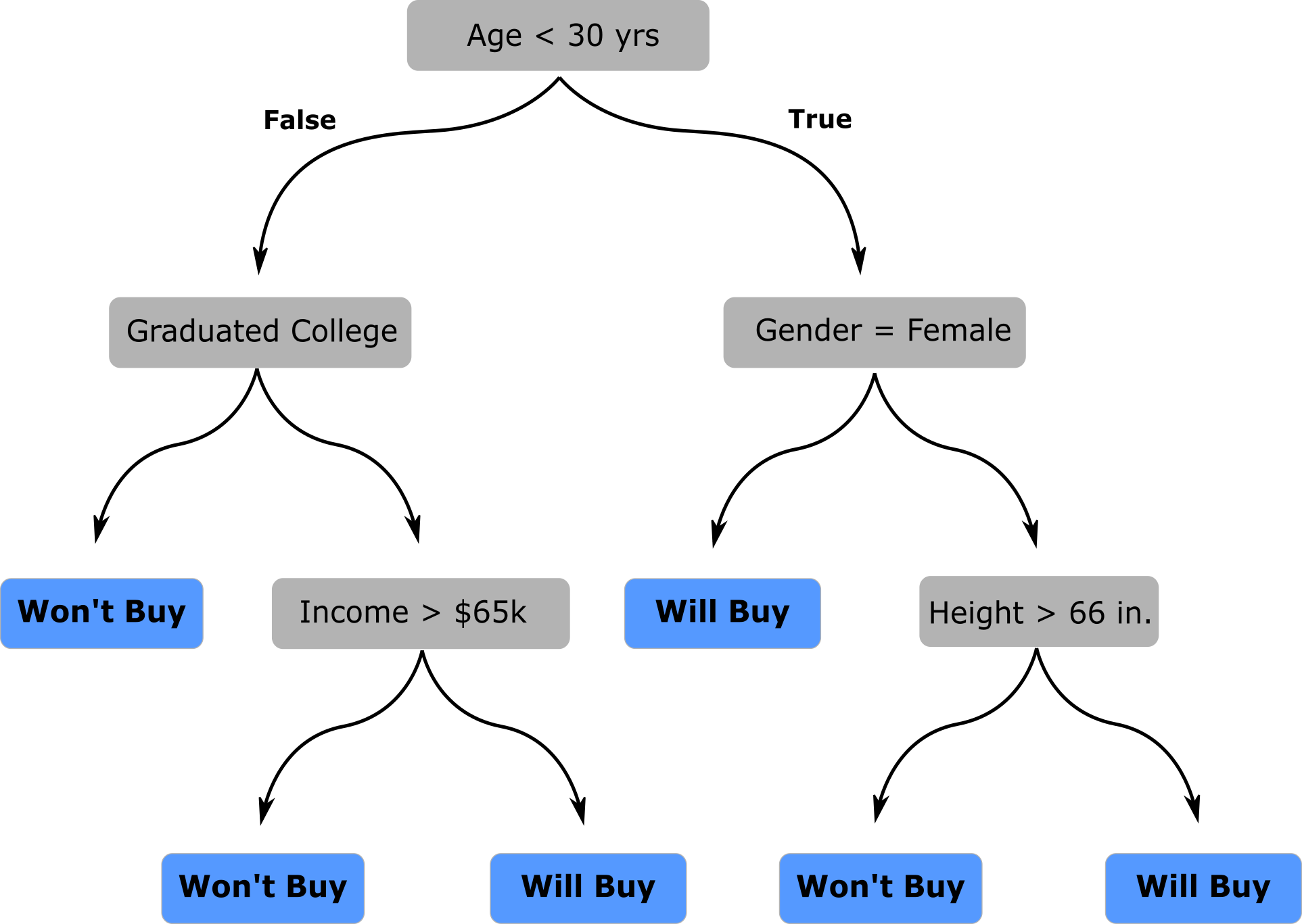
In order to utilize this tree to make a prediction on the outcome of a new sales lead, we start at the root node and apply the statement to our data: Is a person younger than 30 years old? If so, follow the branch to the right, if not, follow the branch to the left. Continue traversing the tree, evaluating the sales opportunity at each decision node. Ultimately, you will arrive at a leaf node that informs you whether the sales opportunity will likely be successful or not. To illustrate, let’s consider we have a new sales opportunity with the following individual:
| Age (yrs) | Gender | Height (in) | College Degree? | Income Estimate |
|---|---|---|---|---|
| 60 | M | 64 | Yes | $50-60k |
Using our decision tree, we can predict that the sales lead is unlikely to be successful and accordingly may not be worth our resources to pursue. The image below shows how the tree was traversed to make that prediction.

Pretty cool, right? But how did we build this tree? And more generally, how do we take an arbitrary training data set and generate the tree structure and associated decisions that we can use for future predictions? We’ll talk about that next.
Decision Tree Learning
The way the algorithm works at its core is to partition the training data set into smaller and mutually exclusive groups through a process called recursive partitioning. Recursive partitioning is just a fancy way of saying splitting the data into subgroups and further splitting those subgroups into additional subgroups. The way the training data is partitioned is by creating a bunch of successive split criteria – which are nothing but the True/False evaluation statements like the ones we saw in the decision nodes in the above tree. The practical problem is the following: how do we know what evaluation criteria to use, and how do we assemble them into a tree-like structure in such a way that the result is useful? For our case, should we first split on age and then on gender? Vice versa? What value of age is the best age to split on? This is where the algorithm comes to our rescue. It builds the tree, starting at the root node, by greedily choosing the best split criteria at each node. This is done by considering every possible split value for every possible feature and then selecting the “best” one as the split criteria. This is why it is called Decision Tree Learning, because the algorithm will actually learn the structure of the tree from the data you give it. This begs the question, though, how do we define the quality of a split?
The most intuitive way to think of the quality of a split is to think about how homogenous (or how pure) the resulting partitions of data are in terms of the outcome your model should predict. The combination of feature and split value that maximize the homogeneity of the resulting partitions is chosen. For those that are interested in reading a little more about the actual metrics used to measure what I am calling “purity” and “homogeneity”, take a look at “Gini Impurity and Information Gain”. This process of selecting the “best” split is repeated starting at the root node and then again on each subsequent node in a recursive fashion until all the data points in a node have the same value or no more splits can be made. Basically, stop splitting when the terminal nodes are 100% pure or there are no more attributes to split. This is known as a “fully grown” decision tree. Fully grown trees, however can be a little problematic as we’ll discuss shortly.
At each leaf node of the tree, use the most common value of the training data labels to assign the predicted value for that node. For example, if you come to a leaf node that has 100 training data points and all were labeled as Successful Sales, create a rule for this node that says any future data that fall into this partition should be predicted to be Successful Sales. If the target variable for the training data in leaf node is not homogeneous, use the more common label from the training data, or better yet assign an estimate of probability. For example, if the leaf node has 70 Successful Sales and 30 Unsuccessful attempts, you could assign future data that falls in that partition to be Successful (this is called a Hard Rule) or you can assign them 70% likely to be Successful (this is called a Soft Rule), to give an indication of the strength of the rule. Generally Soft Rules are preferable because they convey more information.
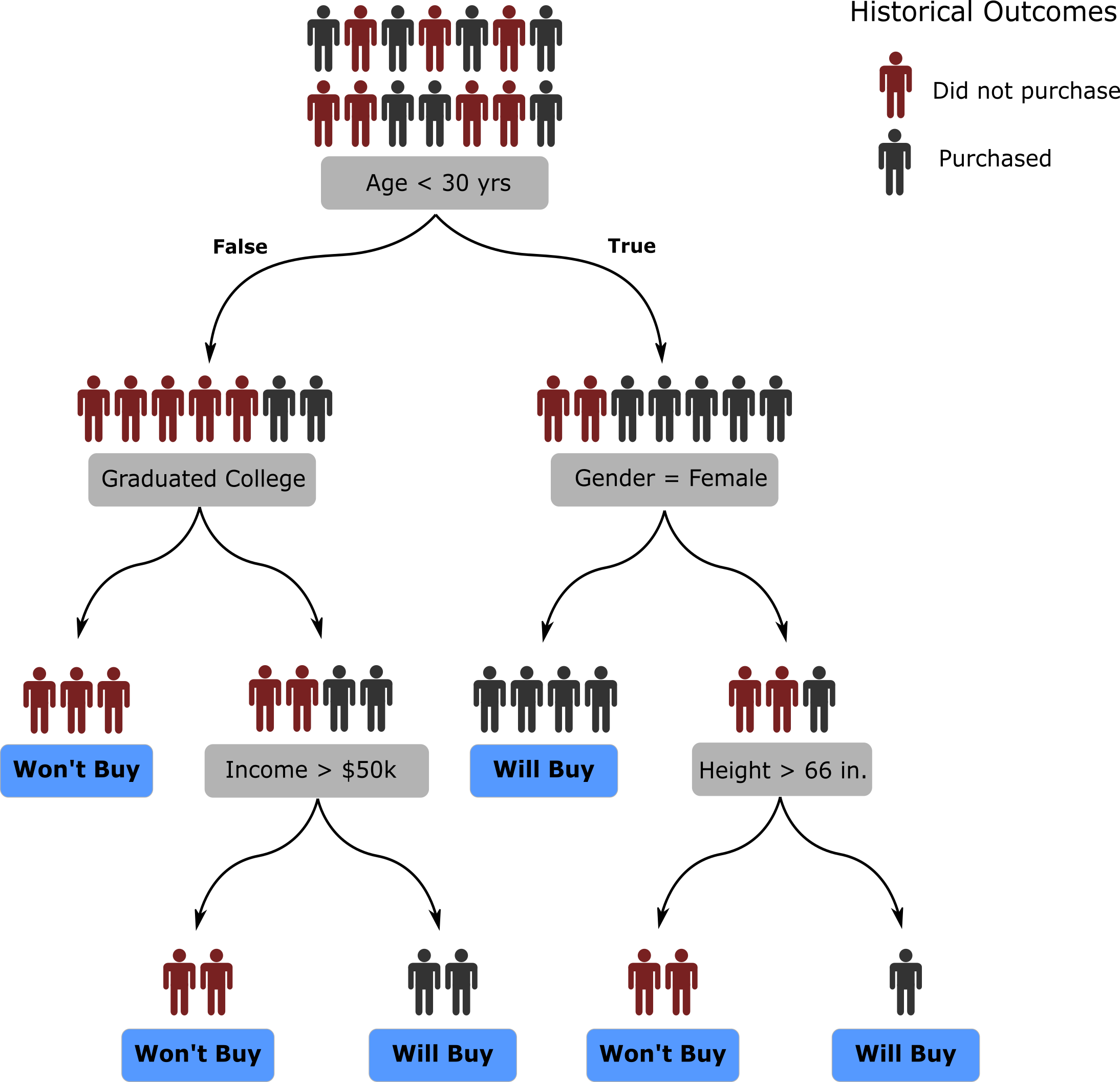
Our decision tree for predicting sales outcomes from above is shown again below, but now, you can see the associated training data that was used to learn the actual tree. Each one of the training samples – representing a historical sales leads – is represented by a black or red stick figure to represent whether the outcome of the lead was a successful sale or not. The more you go down the tree the more homogenous the groups become.
Practical Considerations
There are some practical considerations when learning a fully-grown decision tree as outlined in the procedure above. To motivate potential shortcomings, consider that the overall objective of building a decision tree is to learn the patterns from your sample of training data to predict something about future samples from the population of data. Specifically, you want to learn about the patterns in your data that generalize to the population of unseen data. Likewise, you want to make sure you don’t learn the specific patterns within your data that are not representative of the patterns in the population – think of this as noise. The question becomes: how do we ensure we are learning as much useful information about our data as possible without learning superfluous patterns specific only to our sample of data? This is commonly referred to as balancing underfitting and overfitting the training data.
The practical approaches to avoiding the issue of your Decision Tree overfitting your training data are to stop partitioning after the tree reaches a certain depth (which can serve to limit the complexity of a partition), stop partitioning after the number of data points in a node drops below some threshold level (limiting the minimum size of a partition), or stop splitting when the gain in “purity” resulting from any additional splits drops below some threshold value. By doing these things, it is often found that the performance of the resulting decision tree will be better on new, unseen data. I wish there was a way that I could tell you what the best tree depth was, or the best minimum leaf node size, but in practice, you’ll need to try various combinations and figure out what works best for your specific problem (that’s called “model tuning”).
Conclusions
In this blog post, I introduced a basic decision tree algorithm, explained how simple and easy to interpret the outputs are. Then I introduced at a high level about how the algorithm builds a decision tree from a set of data. I used a simple toy case to demonstrate some of the concepts, but in practice, decision trees can accommodate much more data. There have been numerous enhancements and extensions of the decision tree algorithm as described above to make them more powerful, but the heart of the algorithm is largely the same. In fact, decision trees formed the algorithmic backbone of the incredible accuracy that the Microsoft’s Xbox Kinect (the camera) has at tracking and identifying body parts. You can read more about that here. I have tried to keep this as nontechnical as possible while still getting the idea across. If I missed the mark or if you’d like to see more technical details in the future feel free to email us at analytics@axisgroup.com or leave a comment.
About Tim:
 Tim is a Data Science Consultant at Axis Group. He has in-depth knowledge of data science, machine learning, business analytics, and business intelligence. He believes that “Data Science” is too often thrown around as a buzz word and hates seeing when the methods used to solve a problem become more important than the problem itself. He is passionate about working with partners to identify the appropriate data analysis techniques – whether the use BI dashboarding, machine learning, statistical models, or any other data approach – to solve their problems efficiently, and in the context of their organizational capabilities. Tim is a two-time graduate of Georgia Tech, having earned a PhD in Civil Engineering and a MS in Analytics.